The world of mathematics is rich with intriguing questions, and one that frequently piques curiosity is: “Which function equation is represented by the graph?” This inquiry transcends mere recognition; it challenges one to delve into the intricate relationship between algebraic expressions and their graphical counterparts. Understanding how to interpret a graph and discern the underlying function is not only essential for mathematical proficiency but also vital for applications across various disciplines, including physics, economics, and engineering. This article endeavors to guide you through the steps necessary to unearth the correct function equation that corresponds to any given graph.
To embark on this mathematical journey, we must first develop a fundamental comprehension of function types. In the realm of functions, several categories prevail, such as linear, quadratic, polynomial, exponential, and logarithmic functions. Each category possesses distinct characteristics that manifest in their graphical representations. Thus, the initial objective is to ascertain which category the graph falls into. Is the graph straight and unwavering, indicative of a linear function? Or does it exhibit a curved trajectory, suggesting a quadratic or perhaps a polynomial function? By making these preliminary observations, one can streamline the pursuit of the correct function equation.
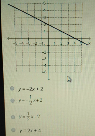
Graphical interpretation begins with identifying key features of the graph. For instance, does the graph intersect the y-axis? If so, the point where it intersects provides a pivotal clue known as the y-intercept. In linear functions, this information is readily incorporated into the slope-intercept form, y = mx + b, where ‘m’ represents the slope and ‘b’ signifies the y-intercept. Such clear-cut identification also facilitates the recognition of linear relationships, making it an excellent starting point for analysis.
Next, consider the slope of the line if you are dealing with a linear function. The steepness and direction of the line—whether it ascends or descends as you progress along the x-axis—are indicative of the slope. A positive slope corresponds to an ascending line, while a negative slope indicates a descending one. By selecting any two points on the line, one can compute the slope using the formula (y₂ – y₁) / (x₂ – x₁). This mathematical exercise solidifies your understanding of the graph’s behavior and further informs the construction of the function equation.
Moving beyond linear functions, one must also consider the possibility of quadratic functions, often represented by parabolas. When confronting a graph that exhibits a distinct ‘U’ shape, the inquiry shifts to the quadratic equation, generally expressed as y = ax² + bx + c. The parameters ‘a’, ‘b’, and ‘c’ are quintessential in determining the location of the vertex and the direction in which the parabola opens. A positive ‘a’ yields a parabola that opens upwards, while a negative ‘a’ results in an opening downwards. In this scenario, identifying the vertex’s x-coordinate—calculated by -b/(2a)—is instrumental in pinpointing the graph’s apex and aligning it with the respective equation.
Polynomial functions weave a different narrative altogether. With increasing degrees, the graphs of polynomials display more complex behaviors, including multiple turning points and varied end-behavior. If observations indicate a graph with two or more bends, or a more intricate path, one might be prompted to consider polynomial equations. The general form of a polynomial function, y = a_n * x^n + a_(n-1) * x^(n-1) + … + a_1 * x + a_0, elaborates upon the variable ‘n’, which denotes the degree of the polynomial. The behavior of the graph at the extremes can also inform which polynomial degree is applicable, giving insights into the equation that governs it.
Exponential functions, which can be recognized by their characteristic rapid growth or decay, deserve attention next. Graphs that ascend rapidly or decrease swiftly as they approach zero typically represent exponential functions, expressed in the format y = ab^x. Key features of exponential graphs include horizontal asymptotes and growth/decay rates determined by the base ‘b’. Analysis of these features will enhance your ability to derive the exponential function equation appropriately.
Logarithmic functions are another consideration, often represented as the inverse of exponential functions. Their graphs are characterized by a gradual increase that approaches a vertical asymptote. When interpreting a logarithmic graph, one can express the function in the form y = a + b log(x). Recognizing the asymptote and growth will crucially guide you in determining the parameters of the function.
Once you have hypothesized the function type that corresponds with the graph, the next step entails validating your assumptions. This validation process often involves substituting known points (coordinates) back into the proposed function equation to verify if they indeed satisfy it. By employing this method, one can confirm whether the graph aligns with the selected function equation or if additional adjustments are necessary.
The culmination of this analytical adventure is the realization that the interplay between a function’s algebraic form and its graphical representation is a beautifully symbiotic relationship. The ability to decode a graph not only fortifies one’s mathematical acumen but also empowers one to navigate complex data visualization challenges with confidence. As the adage goes, “A picture is worth a thousand words,” and in mathematics, a graph may very well represent a myriad of function equations, just waiting for an astute observer to uncover them. With practice, patience, and a robust understanding of these principles, you will not only discover the function equation represented by any graph you encounter, but you may also find your appreciation for the mathematical world deepening significantly.

Leave a comment